Electrostatics

Charging and the flow of charge

Ordinary matter contains positively charged nuclei and negatively charged electrons. Most nuclei also contain neutral neutrons. Charging everyday objects mainly involves moving electrons between them. A proton has charge $+e$, an electron has charge $-e$, and a neutron is neutral, where

$$e=1.602\times 10^{-19}\text{ C}.$$

This is the elementary charge. An object becomes negative by gaining electrons and positive by losing them. Charging redistributes charge; it does not create net charge. The total charge of an isolated system stays constant.

How that excess charge moves depends on the material:

• Conductors have mobile charges that can redistribute through the material.
• Insulators have charges that are locally bound, so charge does not freely flow through the object.
• Semiconductors are between the two: they have some mobile charge carriers, but far fewer than a good conductor.

This difference matters when we charge an object. In conduction, objects make electrical contact and electrons move between them. Two connected conductors reach the same potential at equilibrium; they do not necessarily end up with equal charges. Identical, widely separated metal spheres are a useful special case: after contact and separation, each has half the original total charge.

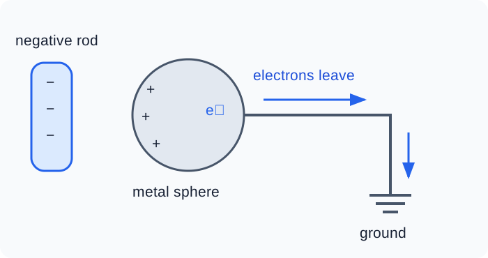
In induction, a nearby charged object changes the charge distribution without touching the conductor. Bring a negative rod near an isolated neutral metal sphere: electrons move to the far side, leaving a positive region near the rod. The sphere is polarized, but its total charge is still zero.

To leave a net positive charge on the sphere, connect it to ground while the negative rod is nearby. Repelled electrons can then leave through the wire. Disconnect the ground first, then remove the rod. The remaining positive charge redistributes over the sphere. Removing the rod while the sphere is still grounded would let electrons return and undo the charging. A positive inducing rod reverses the charge signs and electron-flow direction.

Grounding connects the conductor to a large charge reservoir, usually Earth. Electrons flow in either direction until the conductor reaches Earth’s potential, which we choose as $V=0$. Grounding fixes potential, not net charge: the nearby rod can leave the grounded sphere positively charged even while it is connected.

---

Electric force and Coulomb’s law

Theorem (Coulomb’s Law). For point-like charges,

$$\vec F = k\frac{q_1q_2}{r^2}\hat r, \qquad k=\frac{1}{4\pi\varepsilon_0}.$$

The force is repulsive for like charges and attractive for opposite charges.

Here $\hat r$ points from source charge $q_1$ toward the charge $q_2$ experiencing the force. The signs of $q_1q_2$ then give the direction. Doubling the separation reduces the force to one quarter; the expression applies to stationary point charges in vacuum, or outside spherically symmetric charge distributions when their centers can be used as the source points.

For several charges, use superposition: each source contributes its own force, and the net force is their vector sum. If a charge $q$ sits at $\vec r$ and source charges $q_i$ sit at $\vec r_i$,

$$\vec F(\vec r)=kq\sum_i q_i\frac{\vec r-\vec r_i}{\lvert\vec r-\vec r_i\rvert^3}.$$

For a continuous distribution, divide the source into small elements $dq$ and replace the sum by an integral:

$$\vec F(\vec r)=kq\int \frac{\vec r-\vec r'}{\lvert\vec r-\vec r'\rvert^3}\,dq.$$

The source coordinate $\vec r'$ varies during integration; the observation point $\vec r$ stays fixed. Resolve directions before integrating. Adding force magnitudes would miss cancellations.

Vacuum permittivity

The constant $\varepsilon_0$, read “epsilon naught,” is the vacuum permittivity. It sets the strength of electric interactions in SI units:

$$\varepsilon_0\approx8.854\times10^{-12}\ \frac{\mathrm C^2}{\mathrm{N\,m}^2} =8.854\times10^{-12}\ \mathrm{F/m}, \qquad k=\frac{1}{4\pi\varepsilon_0}\approx8.988\times10^9\ \frac{\mathrm{N\,m}^2}{\mathrm C^2}.$$

The factor $4\pi$ comes from the geometry of a sphere, which has area $4\pi r^2$. We will see it cancel when integrating a point charge’s field over a spherical surface in Gauss’s law.

In a uniform, linear, isotropic dielectric filling the region, we often use $\varepsilon=\varepsilon_r\varepsilon_0$. Interfaces and nonuniform materials require more care because polarization adds bound charges; those effects are covered in the capacitor and dielectric notes.

Example. Two charges $+Q$ are fixed at $(a,0)$ and $(-a,0)$. A charge $-q$, with $q>0$, is at $(0,b)$, where $b>0$. Find the net force on $-q$.

Both source charges attract it. Their horizontal forces cancel, and both vertical components point down. Each separation is $d=\sqrt{a^2+b^2}$, so

$$F_y=-2\left(\frac{kQq}{d^2}\right)\frac{b}{d} =-\frac{2kQqb}{(a^2+b^2)^{3/2}}, \qquad F_x=0.$$

For $b\gg a$ this approaches $-2kQq/b^2$, the force of a single charge $2Q$ at the origin.

Electric fields

An electric field assigns a vector to every point in space. That vector tells us the force a positive unit charge would experience there. The source charges establish the field whether or not we place a test charge at that point.

This separates the source configuration from the particle responding to it: calculate $\vec E$ once, then use $\vec F=q\vec E$ for any test charge. A negative charge feels a force opposite the field. The test charge must be small enough that it does not appreciably rearrange the sources.

The electric field is force per unit positive test charge:

$$\vec E=\frac{\vec F}{q_0}.$$

Since the electric field is a vector, it can be broken down into components:

$$\vec E(x,y,z)=E_x(x,y,z)\hat i+E_y(x,y,z)\hat j+E_z(x,y,z)\hat k.$$

In addition, by the superposition principle, for many source charges, add the individual fields:

$$\vec E_{\text{net}}=\sum_i \vec E_i.$$

For continuous charge distributions, we can replace the sum by an integral:

$$dE=k\frac{dq}{r^2},$$

where

$$dq=\lambda\,d\ell,\qquad dq=\sigma\,dA,\qquad dq=\rho\,dV.$$

It is very important to choose useful coordinates (e.g. rectangular, polar, spherical, etc.), use symmetry to cancel components, project the remaining component, then integrate.

Example. Find the electric field of a uniformly charged disk with radius $R$ at a point $x$ above the center.

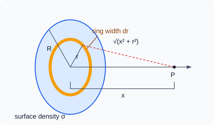
A uniformly charged disk can be built from thin rings. If the disk has surface charge density $\sigma$, then a ring of radius $r$ and thickness $dr$ has

$$dq=\sigma(2\pi r\,dr).$$

Using the on-axis field of a thin ring — a ring of charge $dq$ at radius $r$ contributes an axial field $k\,x\,dq/(x^2+r^2)^{3/2}$ (this ring result is derived cheaply from the potential in the potential section below),

$$dE_x=k\frac{x\,dq}{(x^2+r^2)^{3/2}} =k\frac{x(2\pi\sigma r\,dr)}{(x^2+r^2)^{3/2}}.$$

Integrating from $r=0$ to $R$ gives

$$E_x=2\pi k\sigma\left(1-\frac{x}{\sqrt{x^2+R^2}}\right) =\frac{\sigma}{2\varepsilon_0}\left(1-\frac{x}{\sqrt{x^2+R^2}}\right)$$

for $x>0$.

Example. A solid hemisphere of radius $R$ occupies $z\ge0$ and has uniform volume charge density $\rho$. Find the electric field at the origin, the center of its flat face, using disks and then a triple integral.

Rotational symmetry cancels the horizontal components. For $\rho>0$ the field points down, away from the charge above the origin.

Method 1: stack thin disks. At height $z$ the disk radius is $\sqrt{R^2-z^2}$, and a slice of thickness $dz$ has effective surface charge density $\rho\,dz$. Apply the disk result to a point a distance $z$ below that slice:

$$dE_z=-\frac{\rho\,dz}{2\varepsilon_0} \left(1-\frac{z}{\sqrt{z^2+(R^2-z^2)}}\right) =-\frac{\rho}{2\varepsilon_0}\left(1-\frac{z}{R}\right)dz.$$

Then

$$E_z=-\frac{\rho}{2\varepsilon_0}\int_0^R\left(1-\frac{z}{R}\right)dz =-\frac{\rho R}{4\varepsilon_0}.$$

Method 2: spherical-coordinate triple integral. Let $r$ measure the source point’s distance from the origin and $\theta$ its angle from $+z$. The hemisphere has $0\le r\le R$, $0\le\theta\le\pi/2$, and $0\le\phi\le2\pi$. Since

$$dq=\rho r^2\sin\theta\,dr\,d\theta\,d\phi,$$

the downward field component is $dE_z=-k\,dq\cos\theta/r^2$. Thus

$$E_z=-k\rho \int_0^Rdr\int_0^{\pi/2}\sin\theta\cos\theta\,d\theta \int_0^{2\pi}d\phi =-k\rho R\left(\frac12\right)(2\pi) =-\frac{\rho R}{4\varepsilon_0}.$$

Both methods give

$$\vec E=-\frac{\rho R}{4\varepsilon_0}\hat z.$$

The apparent $1/r^2$ singularity cancels against the volume element, so the integral remains finite at the origin.

---

Electric field lines

Field lines are a visual tool:

• They begin on positive charge and end on negative charge.
• They point in the direction of $\vec E$.
• Their density represents field strength.
• They never cross, because the field at one point cannot have two directions.

Field lines are not the field itself. They are a way to visualize a vector field in space.

// note to self: add the hw problem about electric field lines (problem 6 of Ran, HW 1)

Electric flux and Gauss’ Law

Electric flux measures how much electric field passes through a surface:

$$\Phi_E=\int \vec E\cdot d\vec A.$$

The direction of $d\vec A$ is the local normal direction. For a closed surface, the outward normal is positive by convention.

For a uniform field through a flat area,

$$\Phi_E=EA\cos\theta.$$

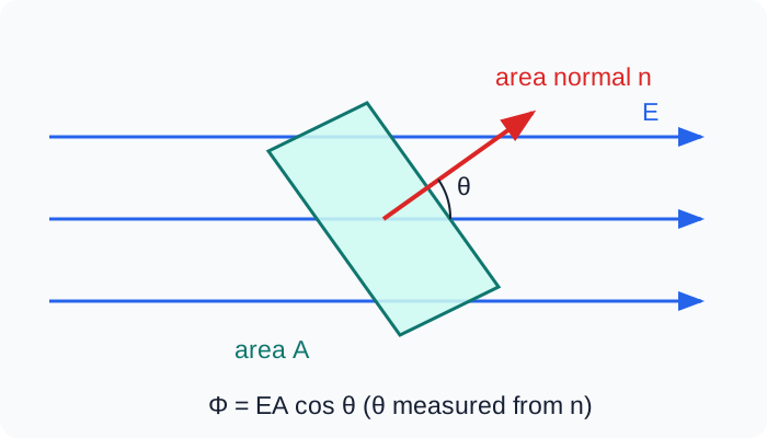
For an open surface, flux depends on its area and orientation. For a closed surface, count outward crossings positively and inward crossings negatively. An external charge can send field through the surface, but its entering and leaving contributions cancel. Gauss’s law makes this connection between net flux and enclosed charge exact:

Theorem (Gauss’s Law). The net electric flux through any closed surface equals the enclosed charge over $\varepsilon_0$,

$$\oint \vec E\cdot d\vec A=\frac{Q_{\text{enc}}}{\varepsilon_0}.$$

Proof (Gauss’s law). First prove the result for one point charge $q$. By Coulomb’s law, the electric field a distance $r$ from the charge is

$$\vec E=k\frac{q}{r^2}\hat r =\frac{1}{4\pi\varepsilon_0}\frac{q}{r^2}\hat r.$$

For a tiny area element $dA$ on any closed surface, only the component of $\vec E$ perpendicular to the surface contributes to flux:

$$d\Phi_E=\vec E\cdot d\vec A =\frac{q}{4\pi\varepsilon_0}\frac{\cos\theta\,dA}{r^2},$$

where $\theta$ is the angle between $\hat r$ and the outward normal. The quantity

$$d\Omega=\frac{\cos\theta\,dA}{r^2}$$

is the solid angle subtended by the area element as seen from the charge. Therefore

$$d\Phi_E=\frac{q}{4\pi\varepsilon_0}\,d\Omega.$$

If the charge is inside the closed surface, the surface surrounds the charge once, so the total solid angle is $4\pi$ steradians (3D equivalent of radians). Hence

$$\oint \vec E\cdot d\vec A =\frac{q}{4\pi\varepsilon_0}\oint d\Omega =\frac{q}{4\pi\varepsilon_0}(4\pi) =\frac{q}{\varepsilon_0}.$$

If the charge is outside the closed surface, field lines that enter the surface also leave it. Equivalently, the signed solid angles cancel, so the net flux is $0$.

For many point charges, electric fields add by superposition:

$$\vec E=\sum_i \vec E_i.$$

Flux is linear, so

$$\oint \vec E\cdot d\vec A =\sum_i\oint \vec E_i\cdot d\vec A.$$

Each charge inside contributes $q_i/\varepsilon_0$, and each charge outside contributes $0$. Thus

$$\oint \vec E\cdot d\vec A =\frac{1}{\varepsilon_0}\sum_{\text{inside}}q_i =\frac{Q_{\text{enc}}}{\varepsilon_0}.$$

A continuous charge distribution is the same argument with the sum replaced by an integral over charge elements $dq$.

Tip

Tip

Good Gaussian surfaces match the symmetry:

• sphere for spherical symmetry,
• cylinder for infinite line/cylindrical symmetry,
• pillbox for infinite plane symmetry.

Example. A nonconducting sphere of radius $R$ has charge density $\rho(r)=\rho_0r/R$. Find its electric field inside and outside.

A concentric Gaussian sphere has constant radial field. For $r<R$, first integrate the charge actually enclosed:

$$Q_{\mathrm{enc}}(r)=4\pi\int_0^r\frac{\rho_0r'}{R}r'^2\,dr' =\frac{\pi\rho_0r^4}{R}.$$

Gauss’s law gives $4\pi r^2E_r=Q_{\mathrm{enc}}/\varepsilon_0$, so

$$E_r(r)= \begin{cases} \rho_0r^2/(4\varepsilon_0R),&r<R,\\ \rho_0R^3/(4\varepsilon_0r^2),&r>R. \end{cases}$$

The total charge is $\pi\rho_0R^3$. The two expressions agree at $r=R$, and the exterior field falls as $1/r^2$.

Standard Gaussian results

// note to self, make sure to every standard E is here

Often times, USAPhO problems rely on standard cases of Gauss’ Law (which you can try to derive yourself!).

For a thin spherical shell of radius $R$ and total charge $Q$,

$$E(r)= \begin{cases} 0, & r<R,\\ kQ/r^2, & r>R. \end{cases}$$

This is the electrostatic version of Newton’s shell theorem.

For a uniformly charged solid sphere of radius $R$ and total charge $Q$,

$$E(r)= \begin{cases} kQr/R^3, & r<R,\\ kQ/r^2, & r>R. \end{cases}$$

For an infinite line of charge,

$$E=\frac{\lambda}{2\pi\varepsilon_0 r}.$$

For an infinite cylindrical shell with charge per unit length $\lambda$,

$$E= \begin{cases} 0, & r<R,\\ \lambda/(2\pi\varepsilon_0 r), & r>R. \end{cases}$$

For an infinite nonconducting plane sheet,

$$E=\frac{\sigma}{2\varepsilon_0}.$$

The direction is perpendicular to the sheet, away from positive charge and toward negative charge.

Feel free to derive these yourself, although the procedures are pretty standard.

Two of these combine constantly. A pair of parallel, oppositely charged sheets $\pm\sigma$ superpose to give a uniform field between them and (ideally) zero field outside:

$$E_{\text{between}}=\frac{\sigma}{\varepsilon_0},\qquad E_{\text{outside}}=0.$$

This is the parallel-plate capacitor field — twice the single-sheet value, because in the gap both sheets push the same way while outside they cancel.

Superposition also cracks a classic that has no symmetry of its own:

Example. A sphere of uniform charge density $\rho$ has a smaller spherical cavity hollowed out of it, the cavity’s center displaced by $\vec d$ from the big sphere’s center. Show that the field everywhere inside the cavity is uniform.

View the hollow object as a superposition: a complete solid sphere of density $+\rho$, plus a smaller sphere of density $-\rho$ filling the cavity. Inside a uniform sphere the field is $\vec E=\dfrac{\rho}{3\varepsilon_0}\vec r$ measured from that sphere’s own center (this is the interior result $E=kQr/R^3$ rewritten with $Q=\rho\cdot\tfrac{4}{3}\pi r^3$). Let $\vec r_1$ and $\vec r_2$ be the position of a field point measured from the big-sphere and cavity centers, so $\vec r_1=\vec r_2+\vec d$. Adding the two contributions inside the cavity,

$$\vec E=\frac{\rho}{3\varepsilon_0}\vec r_1-\frac{\rho}{3\varepsilon_0}\vec r_2=\frac{\rho}{3\varepsilon_0}(\vec r_1-\vec r_2)=\frac{\rho}{3\varepsilon_0}\vec d.$$

The field point $\vec r$ cancels, leaving the same field everywhere in the cavity: a uniform field $\dfrac{\rho}{3\varepsilon_0}\vec d$ parallel to the displacement $\vec d$.

Electrostatic equilibrium in conductors

In USAPhO, many problems will deal with conductors, since it is the easiest type of material to model charge transfer and effects on. In a conductor at electrostatic equilibrium, charges have stopped moving macroscopically. Therefore:

• $\vec E=0$ inside the conducting material.
• Excess charge lies on the conductor’s surface.
• The electric field just outside the surface is perpendicular to the surface.
• Larger surface charge density means a stronger field just outside.

If a tangential electric field existed on the surface, free charge would slide along the conductor, so equilibrium would not hold.

For a conductor surface with local surface charge density $\sigma$,

$$E_{\text{outside}}=\frac{\sigma}{\varepsilon_0}.$$

These features are very important to remember for any conductor problems, since it makes it so much easier to solve. In addition, the outward electrostatic pressure on a charged conducting surface is

$$P=\frac{\sigma^2}{2\varepsilon_0}.$$

One way to remember this is that the surface charge feels the field from the rest of the conductor, not the full field including itself; that gives the factor of $1/2$.

Example. An isolated conducting sphere of radius $R$ carries charge $Q$ in vacuum. Find its surface charge density, the field immediately outside, and the electrostatic pressure.

Spherical symmetry makes the charge uniform:

$$\sigma=\frac{Q}{4\pi R^2},\qquad \vec E(R^+)=\frac{Q}{4\pi\varepsilon_0R^2}\hat r.$$

The outward pressure is

$$P=\frac{\sigma^2}{2\varepsilon_0} =\frac{Q^2}{32\pi^2\varepsilon_0R^4}.$$

Doubling the charge quadruples the pressure. At fixed charge, doubling the radius reduces the pressure by a factor of $16$. The pressure is outward for either sign of $Q$.

Conducting cavities

A cavity inside a conductor is a useful place to apply Gauss’s law carefully. Draw a Gaussian surface lying entirely inside the conducting material and wrapped tightly around the cavity wall. Since $\vec E=0$ everywhere in the conducting material,

$$\oint \vec E\cdot d\vec A=0 \quad\Longrightarrow\quad Q_{\text{enc}}=0.$$

Therefore, the total charge on the inner cavity surface plus any charge placed inside the cavity must add to zero. If a charge $q$ sits inside the cavity, the inner wall carries total charge $-q$. The outer surface then carries whatever charge is required by the conductor’s total charge.

For an isolated neutral conductor with a cavity charge $q$:

$$Q_{\text{inner}}=-q,\qquad Q_{\text{outer}}=+q.$$

If the same conductor is grounded, charge can flow to Earth. The inner wall still carries $-q$, but the outside does not need to carry $+q$; for a fully shielding grounded conductor, the exterior field can be zero.

Warning

Do not confuse “field inside the conducting material is zero” with “potential is zero.” The conductor is one equipotential, but that constant is only zero if the conductor is grounded or chosen as the reference.

Example. An isolated conducting shell has total charge $+3q$. A point charge $-q$ sits off-center inside its closed cavity. Find the total charges on the inner and outer surfaces. Then find those totals after grounding the shell, assuming no external charges.

A Gaussian surface inside the metal has zero flux, so the inner wall must cancel the cavity charge:

$$Q_{\mathrm{inner}}=+q.$$

Before grounding, charge conservation gives

$$Q_{\mathrm{outer}}=3q-Q_{\mathrm{inner}}=2q.$$

Grounding fixes the shell potential at zero. With no external sources, the exterior solution is $V=0$, so the outer surface becomes uncharged. The inner surface still carries $+q$. The conductor’s total charge changes from $3q$ to $q$, so electrons with total charge $-2q$ have arrived from Earth.

The off-center position makes the inner surface charge nonuniform, but it does not change its total.

---

Electric potential and potential energy

Review: Conservative forces

A force is conservative if the work it does between two points is path-independent, i.e.

$$W=\int_A^B \vec F\cdot d\vec\ell$$

depends only on the endpoints $A$ and $B$. Equivalently,

$$\oint \vec F\cdot d\vec\ell=0 \qquad\Longleftrightarrow\qquad \vec F=-\nabla U$$

for some scalar potential energy $U$. Defining $\Delta U=U(B)-U(A)=-W$ then guarantees mechanical energy conservation, $\Delta E_k+\Delta U=0$, since the work–energy theorem gives $\Delta E_k=W$. Only differences in $U$ are physical; you must fix a reference where $U=0$, and that choice is arbitrary.

Proof (Coulomb force is conservative). Move a charge $q$ from $A$ to $B$ in the field of a fixed charge $Q$ at the origin. Since $\hat r\cdot d\vec\ell=dr$,

$$W=\int_A^B k\frac{Qq}{r^2}\hat r\cdot d\vec\ell =\int_{r_A}^{r_B} k\frac{Qq}{r^2}\,dr =kQq\left(\frac{1}{r_A}-\frac{1}{r_B}\right),$$

which depends only on the initial and final distances and not the path. For a system of source charges, superposition makes the total work the sum of pairwise works, each of which is path-independent, so the total is path-independent too.

Potential energy and potential

For a charge $q$ in the field of a fixed $Q$ with the reference at infinity, $U(r)=kQq/r$. In a general field, pick a reference point $O$ with $U_O=0$:

$$E_p(A)=-\int_O^A q\vec E\cdot d\vec\ell .$$

The minus sign comes from the definition of potential energy: work done by the electric force reduces the stored potential energy. In a small displacement,

$$dU=-dW=-\vec F\cdot d\vec\ell=-q\vec E\cdot d\vec\ell.$$

Integrating from the chosen reference $O$ gives the expression above; $E_p$ is another notation for $U$. For a point source $Q$, choose infinity as the reference and a radial path:

$$U(r)-U(\infty) =-\int_\infty^r\frac{kQq}{r'^2}\,dr' =-kQq\left[-\frac1{r'}\right]_\infty^r =\frac{kQq}{r}.$$

For like charges this is positive: bringing them together requires positive external work. For opposite charges it is negative: the electric force does positive work as they approach.

The electric potential is defined as the energy per unit charge,

$$V(A)=\frac{E_p}{q}=-\int_O^A \vec E\cdot d\vec\ell, \qquad V=\frac{kQ}{r}\ \text{(point charge)} .$$

As opposed to electric field, electric potential is a scalar, meaning that it superposes by ordinary addition, and for continuous distributions it becomes an integral:

$$V=k\sum_i\frac{q_i}{r_i}, \qquad V=k\int\frac{dq}{r}.$$

When the field is already known from symmetry, it is usually faster to integrate it: $\Delta V=-\int \vec E\cdot d\vec\ell$. Although $\vec E$ may jump across a charged surface, but $V$ is always continuous, because it is the integral of a bounded field across zero thickness.

Like potential energy, electric potential requires a reference point. For real (finite) charge distributions, $V(\infty)=0$ is always valid. However, for idealized infinite distributions (e.g. an infinite line or plane) $V=k\int dq/r$ diverges since the source itself extends out to the reference point. There you must choose a finite reference, and can only track changes in potential with respect to a finite point.

Example. Find the field on the axis of a uniformly charged ring of radius $R$ and charge $Q$.

The field integral requires projecting every element onto the axis. The potential integral does not: every element of the ring is the same distance $r=\sqrt{x^2+R^2}$ from the axial point $x$, so the “constant $r$” shortcut gives the answer with no integration at all,

$$V(x)=\frac{k}{r}\int dq=\frac{kQ}{\sqrt{x^2+R^2}} .$$

On the axis, symmetry makes $\vec E$ point along $x$, so the single derivative recovers the full field:

$$E_x=-\frac{dV}{dx}=\frac{kQx}{(x^2+R^2)^{3/2}} .$$

This matches the vector field integral with less calculation. To find $\vec E$ along a symmetry axis, it can be easier to compute the scalar $V$ first and differentiate. Keep $V$ as a function of position until after taking the derivative.

Solving Potentials

• Uniform field: $\Delta V=-\vec E\cdot \vec d$.
• Center of a uniformly charged hemispherical shell (radius $R$, charge $Q$): every element sits at distance $R$, so $V=\frac{k}{R}\int dq=\frac{kQ}{R}$. The same “constant $r$” trick gives the full shell.
• Spherical shell: $V=kQ/r$ outside, $V=kQ/R$ (constant) inside.
• Solid sphere (radius $R$): outside $kQ/r$; inside, integrating the interior field $E=kQr/R^3$ gives $V(r)=\dfrac{kQ}{2R}\left(3-\dfrac{r^2}{R^2}\right)$.
• Coaxial cylinders, linear densities $\pm\lambda$, radii $R_A<R_B$: $V_A-V_B=\dfrac{\lambda}{2\pi\varepsilon_0}\ln\dfrac{R_B}{R_A}$.
• Parallel planes $\pm\sigma$ separated by $d$: $\Delta V=\dfrac{\sigma d}{\varepsilon_0}$.

If you want, it is a good exercise to derive these yourself!

Problem-solving tips

A few habits that save the most time on potential problems:

Tip

Tip

• Reach for the scalar first. Potential adds without components, so $V=k\int dq/r$ is almost always easier than the field integral. If you ultimately need $\vec E$ on a symmetry axis, find $V$ and take $-\nabla V$ (as in the ring example above).
• Look for “constant $r$.” If every charge element is equidistant from the field point (e.g. the center of a ring, shell, arc, or hemisphere) the integral collapses to $V=kQ/r$ with no work.
• If you already have $\vec E$, integrate it, don’t re-integrate $dq$. Once Gauss’s law has given $\vec E$, use $\Delta V=-\int\vec E\cdot d\vec\ell$ along the simplest path (usually radial, so $\vec E\cdot d\vec\ell=E\,dr$).
• Choose the reference to kill terms. Use $V(\infty)=0$ for localized charge; for an infinite line or plane pick a convenient finite point and track only differences.
• Use continuity of $V$ as a free check. When you stitch together piecewise regions (inside/outside a shell, across a boundary), the pieces must agree in value even where $\vec E$ jumps. A mismatch means an algebra error.

Equipotential surfaces and the gradient

Since $V$ is an integral, we can rewrite it the total differential and comparing it with $dV=-\vec E\cdot d\vec\ell$ can give us the electric field components:

$$dV=\frac{\partial V}{\partial x}dx+\frac{\partial V}{\partial y}dy+\frac{\partial V}{\partial z}dz=-E_x\,dx-E_y\,dy-E_z\,dz,$$

so $E_x=-\partial V/\partial x$ (and likewise for $y,z$), i.e. $\vec E=-\nabla V$. The field is the negative gradient of the potential: it points in the direction of steepest decrease of $V$, with magnitude equal to that steepest slope.

An equipotential surface is defined as a surface of constant $V$. These surfaces have two main properties:

• Field lines cross equipotentials at right angles. Moving a charge along an equipotential changes $V$ by zero, so $\vec E\cdot d\vec\ell=0$ for any step within the surface; the field has no tangential component and is therefore perpendicular to the surface. (Equivalently, no work is done moving a charge along an equipotential.)
• Closely spaced equipotentials mean a strong field. Since $E$ is the rate of change of $V$ with distance, tightly packed surfaces — a large $\Delta V$ over a small distance — signal a large gradient and a strong field.

The surface of a conductor in equilibrium is itself an equipotential, which is exactly why field lines always meet a conductor perpendicularly.

Example. In a region of space, $V(x,y)=A(x^2-y^2)$, where $A>0$ has units $\mathrm{V/m^2}$. Find the field and show that it is perpendicular to the equipotential through $(a,a)$, where $a>0$.

Taking the negative gradient,

$$\vec E=-2Ax\,\hat i+2Ay\,\hat j.$$

At $(a,a)$, the potential is zero. The local equipotential is the line $y=x$, with tangent $\hat t=(\hat i+\hat j)/\sqrt2$. Thus

$$\vec E(a,a)\cdot\hat t =\frac{-2Aa+2Aa}{\sqrt2}=0.$$

The field is perpendicular to the line and has magnitude $2\sqrt2 Aa$. Potential zero at a point does not imply field zero there.

Example. Two thin concentric spherical shells carry charge $Q_1$ (radius $a$) and $Q_2$ (radius $b>a$). Find $V(r)$ everywhere, with $V(\infty)=0$.

Step 1 — field by Gauss’s law in each region. Only enclosed charge matters:

$$E(r)= \begin{cases} 0, & r<a,\\[1mm] kQ_1/r^2, & a<r<b,\\[1mm] k(Q_1+Q_2)/r^2, & r>b. \end{cases}$$

Step 2 — integrate inward from infinity. For $r>b$,

$$V(r)=\frac{k(Q_1+Q_2)}{r}.$$

Step 3 — fix the next constant by continuity at $r=b$. In $a<r<b$, integrating $E=kQ_1/r^2$ gives $V=kQ_1/r+C$. Matching to the outer solution at $r=b$,

$$\frac{kQ_1}{b}+C=\frac{k(Q_1+Q_2)}{b} \quad\Longrightarrow\quad C=\frac{kQ_2}{b}, \qquad V(r)=\frac{kQ_1}{r}+\frac{kQ_2}{b}.$$

Step 4 — inside the inner shell. Here $E=0$, so $V$ is constant, equal to its value at $r=a$:

$$V(r<a)=\frac{kQ_1}{a}+\frac{kQ_2}{b}.$$

Each integration constant was pinned down by demanding $V$ be continuous at a boundary—the free check from the tips list, now doing real work.

---

Energy of a charge configuration

What if instead of bringing about a new object, we wanted to calculate the energy of a charged configuration? There are three equivalent ways to compute the total potential energy stored in a configuration; choose whichever matches the problem.

1. Pairwise sum. Add the interaction energy of every distinct pair,

$$U=\frac{1}{4\pi\varepsilon_0}\sum_{i<j}\frac{q_iq_j}{r_{ij}} .$$

This excludes the (infinite) self-energy of idealized point charges. The method works because due to the conservativeness of the Coulomb force it doesn’t matter what order you bring in the charges. However, this method is not typically used because it gets messier quickly as the number of charges increases.

2. Charge times potential, halved. Writing $\sum_i q_iV_i$ counts each pair twice, so

$$U=\frac{1}{2}\sum_i q_iV_i \qquad\Longrightarrow\qquad U=\frac{1}{2}\int V\,dq$$

for a continuous distribution, where $V$ is the potential of the whole distribution. Unlike the pairwise sum, this form includes self-energy (energy required to assemble the system against electrostatic repulsion).

3. Charge it up. Assemble the charge from zero, tracking $V$ as a function of the accumulated charge, and integrate $U=\int V\,dq$. This is most used when symmetry keeps the object near one potential as it charges: for instance a conductor, or a sphere built up shell by shell.

4. Field energy The field-energy viewpoint, $U=\int \tfrac12\varepsilon_0E^2\,dV$, is itself a fourth way to compute configuration energy.

Example. What is the potential energy of a solid sphere with radius $R$ and total charge $Q$ (evenly distributed)?

Build the sphere up shell by shell at fixed density $\rho$. When the assembled charge is $q$ at radius $r$ (final radius $R$), $q=Q(r/R)^3$, and the next shell $dq=Q\,\dfrac{3r^2}{R^3}dr$ is brought from infinity to the surface, which sits at $V=kq/r=kQr^2/R^3$. Hence

$$dU=V\,dq=\frac{kQr^2}{R^3}\cdot\frac{3Qr^2}{R^3}\,dr =\frac{3kQ^2}{R^6}r^4\,dr,$$ $$U=\int_0^R \frac{3kQ^2}{R^6}r^4\,dr=\frac{3}{5}\frac{kQ^2}{R}.$$

Example. Find the potential energy of a disk of radius $R$ with uniform surface density $\sigma=Q/\pi R^2$.

Sub-result — potential at the rim. First find the potential at a point $P$ on the edge of a uniform disk of radius $s$. Put the origin at $P$ and use plane polar coordinates $(\rho,\varphi)$ measured from the line through the center. The far boundary of the disk is the circle of radius $s$ centered a distance $s$ away, which in these coordinates is $\rho=2s\cos\varphi$ for $\varphi\in[-\tfrac\pi2,\tfrac\pi2]$. Then

$$V_{\text{rim}}(s)=k\sigma\!\int_{-\pi/2}^{\pi/2}\!\!\int_0^{2s\cos\varphi}\frac{1}{\rho}\,\rho\,d\rho\,d\varphi =k\sigma\!\int_{-\pi/2}^{\pi/2}\!2s\cos\varphi\,d\varphi =4k\sigma s .$$

The $1/\rho$ from Coulomb cancels the $\rho$ in the area element—this cancellation is exactly why the rim point is tractable while a generic interior point gives an elliptic integral.

Build the disk up from the edge. Grow the disk at constant $\sigma$ by depositing successive rings at the current rim. When the disk has radius $s$, the new ring $dq=\sigma(2\pi s)\,ds$ lands at potential $V_{\text{rim}}(s)$, so

$$dU=V_{\text{rim}}(s)\,dq=(4k\sigma s)(2\pi\sigma s\,ds)=8\pi k\sigma^2 s^2\,ds,$$ $$U=\int_0^R 8\pi k\sigma^2 s^2\,ds=\frac{8\pi k\sigma^2 R^3}{3} =\frac{8}{3\pi}\,\frac{kQ^2}{R},$$

after substituting $\sigma=Q/\pi R^2$. The coefficient $8/3\pi\approx0.85$ is larger than the solid sphere’s $3/5$ and the conducting sphere’s $1/2$: flattening the same charge into a disk packs it closer together, raising the stored energy. Note the assembly order does not affect the answer — the same $U$ comes from $\tfrac12\int V\,dq$ over the finished disk, but that route needs the much harder interior potential.

---

Method of images

The method of images introduces fake charges placed outside the physical region. The key idea is that a grounded conductor has fixed potential $V=0$. If you can place imaginary charges so that the conductor surface is also at $V=0$, then the field in the real region matches the actual conductor potential.

This works because of the uniqueness theorem: if a region is bounded by surfaces of specified potential (conductors, or infinity) and the charge in the region’s interior is specified, then the potential throughout the region is unique. So any candidate that (i) obeys Gauss’s law and the loop law and (ii) matches every boundary condition must be the answer — there is no other. If some arrangement of fictitious “image” charges reproduces the correct boundary potential, the field it gives in the real region is guaranteed correct.

For a grounded plane $z=0$ and a real charge $q$ at $(x_0,y_0,a)$ with $a>0$, use

$$q'=-q,\qquad \vec r'=(x_0,y_0,-a).$$

Reflect the charge’s position across the plane and reverse its sign. The image is only a mathematical replacement for the conductor in the region $z>0$; it is not a real charge inside the metal.

For a grounded sphere of radius $R$ centered at the origin, with a real charge $q$ at $\vec r_0=d\hat n$ and $d>R$, use

$$q'=-q\frac{R}{d},\qquad \vec r'=\frac{R^2}{d}\hat n=\frac{R^2}{d^2}\vec r_0.$$

The image lies inside the sphere along the line to the real charge. For any surface point $\vec r$ with $\lvert\vec r\rvert=R$,

$$\lvert\vec r-\vec r'\rvert=\frac{R}{d}\lvert\vec r-\vec r_0\rvert,$$

so $kq/\lvert\vec r-\vec r_0\rvert+kq'/\lvert\vec r-\vec r'\rvert=0$ everywhere on the surface. These values assume grounding. An isolated sphere with prescribed total charge requires an additional image at its center.

Example. A charge $+q$ is a distance $a$ above an infinite grounded conducting plane. Find the force induced on the charge.

Replace the plane by an image charge $-q$ a distance $a$ below the plane.

At every point on the plane, the distances to $+q$ and $-q$ are equal, so their potentials cancel:

$$V=k\frac{q}{r}+k\frac{-q}{r}=0.$$

Thus the image-charge setup satisfies the grounded-plane boundary condition. The force on the real charge equals the Coulomb attraction to the image charge:

$$F=k\frac{q^2}{(2a)^2} =\frac{kq^2}{4a^2},$$

directed toward the conducting plane.

The image also gives the surface charge density on the real plane. Put the real charge at $(0,0,a)$ and the grounded plane at $z=0$. Just above the conductor, the normal field is the $z$-component of the field from the real charge plus image charge:

$$E_z(\rho,0^+) =-\frac{1}{4\pi\varepsilon_0}\frac{2qa}{(\rho^2+a^2)^{3/2}},$$

so

$$\sigma(\rho)=\varepsilon_0E_z =-\frac{qa}{2\pi(\rho^2+a^2)^{3/2}}.$$

Integrating this over the whole plane gives total induced charge $-q$, as expected for a grounded infinite plane. The potential energy of the real charge-conductor system is not simply $kq(-q)/(2a)$; that would double-count the conductor response. The correct energy is half the real-charge/image interaction:

$$U=-\frac{kq^2}{4a}.$$

Example. // note to self: use a Ran problem

---

Problem-solving strategy

Problem-solving strategy

1. A handful of discrete point charges, want force or field: Coulomb’s law $\vec F=k\dfrac{q_1q_2}{r^2}\hat r$ with vector superposition $\vec E_{\text{net}}=\sum_i\vec E_i$. Resolve into components or use symmetry to kill a direction before adding — never sum magnitudes.
2. The distribution has spherical, cylindrical, or planar symmetry: Gauss’s law $\oint\vec E\cdot d\vec A=\dfrac{Q_{\text{enc}}}{\varepsilon_0}$ with the matching Gaussian surface (sphere/cylinder/pillbox). Reach for the memorized shell, solid-sphere, line, and sheet ($E=\sigma/2\varepsilon_0$) results rather than re-deriving.
3. A continuous blob with no useful symmetry: Integrate. Set $dq=\lambda\,d\ell$, $\sigma\,dA$, or $\rho\,dV$, pick good coordinates, project the surviving component, then integrate $dE=k\,dq/r^2$. You may need to do double or even triple integrals.
4. You only need a speed, closest approach, or escape condition: Energy, not force. The Coulomb force is conservative, so $\Delta K=-\Delta U$ with $U=kQq/r$ (reference at infinity for localized charge) collapses the problem to its endpoints.
5. You need $\vec E$ on a symmetry axis, or any field where the geometry is messy: Compute the scalar $V=k\int dq/r$ first (it adds without components), then take $\vec E=-\nabla V$. Watch for the “constant $r$” shortcut (ring/shell/arc) that makes the integral trivial.
6. A conductor is involved: Inside, $\vec E=0$ and the surface is an equipotential; just outside, $E=\sigma/\varepsilon_0$ (perpendicular). For a charge near a grounded plane or sphere, replace the conductor with an image charge that pins the surface to $V=0$, then treat it as a point-charge problem.
7. You need total stored energy: Pick the form that matches the symmetry — pairwise sum $\dfrac{1}{4\pi\varepsilon_0}\sum_{i<j}\dfrac{q_iq_j}{r_{ij}}$ (excludes self-energy), $\tfrac12\int V\,dq$ or “charge it up” $\int V\,dq$ (includes it), or the field integral $\int\tfrac12\varepsilon_0E^2\,dV$ when no symmetry helps with potentials.

Capacitance, electric dipoles, polarization, and dielectric fields continue in Capacitors and Dielectrics.