Magnetism

Magnetic interactions and field lines

A bar magnet has two poles: like poles repel and opposite poles attract. Cutting it in half gives two smaller magnets, each with both poles, rather than an isolated north or south pole. No isolated magnetic monopole has been observed.

Different materials respond differently. Magnetite can be naturally magnetized; some materials become magnetized near another magnet; others respond so weakly that the effect is hard to notice.

For calculations, use fields and currents instead of treating the poles as separate magnetic charges. Moving charges produce magnetic fields and experience magnetic forces. Intrinsic magnetic moments, such as electron spin, also contribute to magnetism in matter.

The magnetic field $\vec B(x,y,z)$ is a vector field with three components. It is also called magnetic induction or magnetic flux density, and its SI unit is the tesla:

$$1\ \text{T}=1\ \frac{\text{N}}{\text{A}\cdot\text{m}}.$$

Field lines are tangent to $\vec B$, with closer spacing representing a stronger field. They do not begin or end on magnetic charges. Around a straight wire they are circles; around a current loop they resemble the field of a bar magnet. They cannot cross where the field has a well-defined nonzero direction. The field exists between the drawn lines too, and a two-dimensional sketch only shows part of a three-dimensional field.

Tip

Tip

A dot $\odot$ means out of the page, like an arrowhead coming toward you. A cross $\otimes$ means into the page, like the tail of an arrow going away.

For the field around a wire, point your right thumb along conventional current; your curled fingers give the field direction.

---

Biot–Savart law

A small current element $I\,d\vec\ell'$ produces a field at an observation point. Define $\vec R=\vec r-\vec r'$ from the source element to that point, with $R=\lvert\vec R\rvert$. Then

$$d\vec B=\frac{\mu_0}{4\pi}\frac{I\,d\vec\ell'\times\hat R}{R^2} =\frac{\mu_0 I}{4\pi}\frac{d\vec\ell'\times\vec R}{R^3}.$$

Here $d\vec\ell'$ points along conventional current, and the permeability of free space is approximately

$$\mu_0\approx4\pi\times10^{-7}\ \text{T}\cdot\text{m/A}.$$

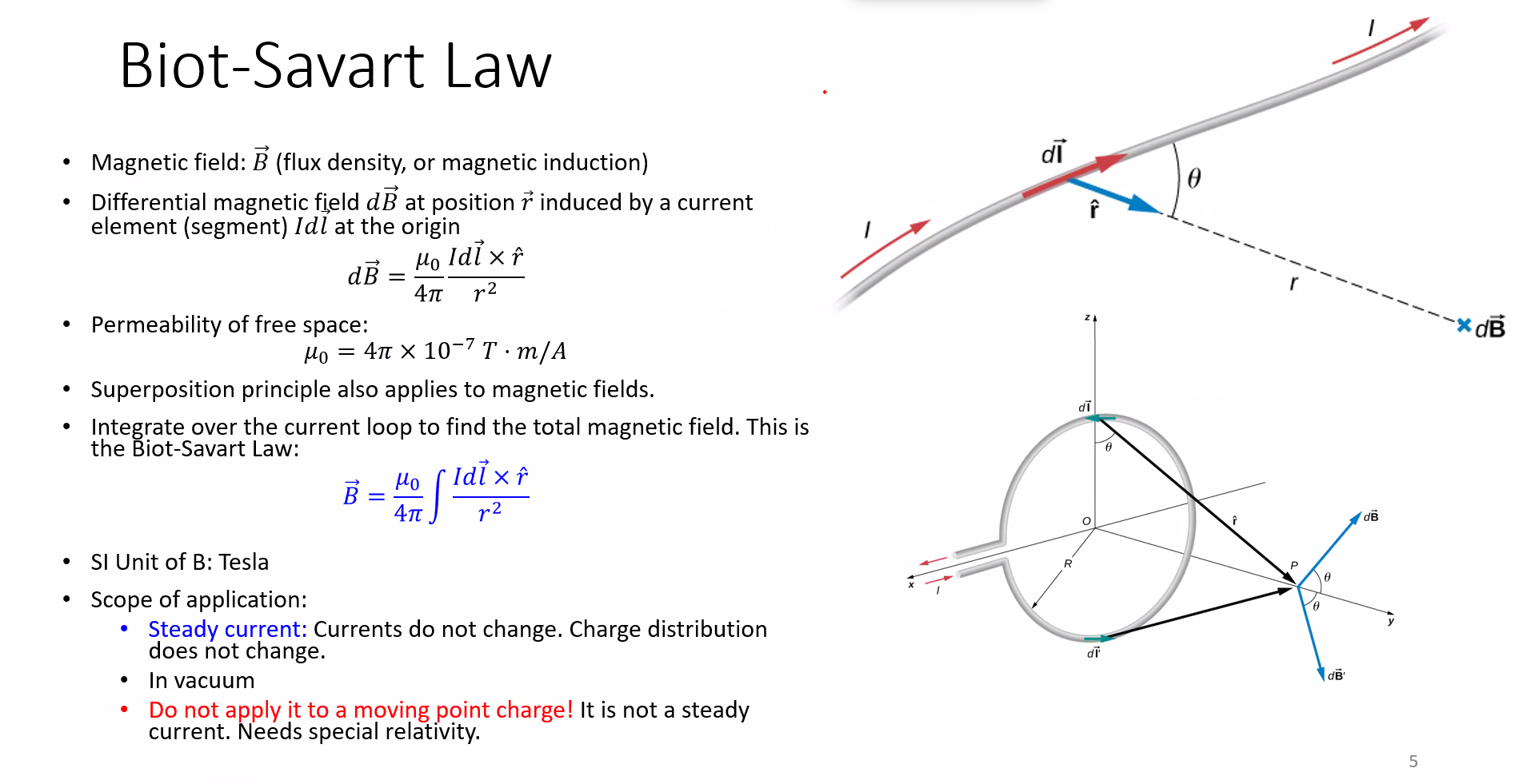
Magnetic fields obey superposition. Add the contributions from every segment of the source circuit:

$$\vec B(\vec r)=\frac{\mu_0 I}{4\pi}\int_C\frac{d\vec\ell'\times\hat R}{R^2}.$$

This is the magnetostatic form: currents and charge distributions are steady. Use it directly for currents in vacuum, or when magnetic effects of the surrounding material can be neglected. A single moving point charge is not a steady current distribution; its general field requires the time-dependent theory, not a direct substitution into this wire formula.

Infinitely long straight wire

Example. An infinitely long wire lies on the $x$-axis and carries current $I$ in the positive $x$ direction. Find the field at $P=(0,a,0)$, where $a>0$.

For a source element at $(x,0,0)$,

$$d\vec\ell'=dx\,\hat x,\qquad \vec R=-x\hat x+a\hat y,\qquad d\vec\ell'\times\vec R=a\,dx\,\hat z.$$

Every contribution points out of the page. Integrating along the wire,

$$\vec B=\frac{\mu_0 I}{4\pi}\int_{-\infty}^{\infty} \frac{a\,dx}{(x^2+a^2)^{3/2}}\,\hat z.$$

Use $x=a\tan\theta$. The integrand becomes $\cos\theta\,d\theta/a$, so

$$\vec B=\frac{\mu_0 I}{4\pi a}\int_{-\pi/2}^{\pi/2}\cos\theta\,d\theta\,\hat z =\frac{\mu_0 I}{2\pi a}\,\hat z.$$

At perpendicular distance $r$ from the wire, the magnitude is $B=\mu_0 I/(2\pi r)$, with direction tangent to a circle around the wire.

Circular current loop

Example. A circular loop of radius $a$ lies in the $xy$-plane and carries current $I$ counterclockwise when viewed from positive $z$. Find its field on the $z$-axis.

Opposite elements give equal and opposite transverse components, leaving only the axial component. Every source element is distance $R=\sqrt{a^2+z^2}$ from the observation point, and

$$dB_z=\frac{\mu_0 I}{4\pi}\frac{a\,d\ell'}{(a^2+z^2)^{3/2}}.$$

Since $\int d\ell'=2\pi a$,

$$\vec B(z)=\frac{\mu_0 I a^2}{2(a^2+z^2)^{3/2}}\,\hat z.$$

At the center,

$$\vec B(0)=\frac{\mu_0 I}{2a}\,\hat z.$$

Reverse the current and the field reverses. For $N$ identical closely stacked turns, multiply by $N$.

Surface and volume currents

For a surface current density $\vec K$, measured in $\text{A/m}$, or a volume current density $\vec J$, measured in $\text{A/m}^2$, replace the wire element by the appropriate distributed-current element:

$$\vec B(\vec r)=\frac{\mu_0}{4\pi}\int_S \frac{\vec K(\vec r')\times\hat R}{R^2}\,dA',$$ $$\vec B(\vec r)=\frac{\mu_0}{4\pi}\int_V \frac{\vec J(\vec r')\times\hat R}{R^2}\,dV'.$$

These integrals can be difficult. Check symmetry before committing to a direct integration: Ampère’s law may give the same field much faster.

---

Magnetic flux and Gauss’s law

Magnetic flux measures the field passing through an oriented surface:

$$\Phi_B=\int_S\vec B\cdot d\vec A.$$

For a uniform field through a flat surface,

$$\Phi_B=BA\cos\theta,$$

where $\theta$ is the angle between the field and the surface normal, not the surface itself. The unit is the weber: $1\ \text{Wb}=1\ \text{T}\cdot\text{m}^2$.

Gauss’s law for magnetism states that the net flux through any closed surface is zero:

$$\oint_S\vec B\cdot d\vec A=0, \qquad \nabla\cdot\vec B=0.$$

Whatever flux enters a closed surface also leaves it. An open surface can have nonzero flux; the closed-surface condition is essential. This is the field-law statement that there are no magnetic monopoles.

Vector potential

A divergence-free magnetic field can be represented using a vector potential $\vec A$:

$$\vec B=\nabla\times\vec A.$$

The identity $\nabla\cdot(\nabla\times\vec A)=0$ makes this consistent with Gauss’s law. Unlike electric potential, $\vec A$ is a vector, not a scalar. It is not unique: adding $\nabla f$ leaves its curl unchanged.

---

Ampère’s circuital law

For steady currents in vacuum,

$$\oint_C\vec B\cdot d\vec\ell=\mu_0 I_{\text{enc}}, \qquad I_{\text{enc}}=\int_S\vec J\cdot d\vec A.$$

Choose a direction around the Amperian loop first. Curl your right-hand fingers in that direction; your thumb gives the positive surface normal. Currents crossing in that direction count positively, and currents crossing the other way count negatively. Use the algebraic sum of enclosed currents.

The law is true for any closed loop in magnetostatics, but it only makes the calculation simple when symmetry tells you enough about $\vec B$. Zero enclosed current means zero circulation, not necessarily zero field everywhere on the loop. Time-dependent fields require the additional displacement-current term; the formulas here use the steady-current limit.

Problem-solving strategy

1. Use symmetry to determine the field’s direction and which coordinates its magnitude can depend on.
2. Choose a loop where $\vec B$ is tangent and constant on useful segments, and perpendicular to the other segments.
3. Calculate the current through the enclosed surface, not just the total current in the entire object.
4. Evaluate the loop integral and solve for the field.

Infinite current sheet

Example. An infinite sheet lies in the $xy$-plane and carries uniform surface current $\vec K=K\hat x$. Find the field on either side.

Symmetry and the right-hand rule give equal field magnitudes: $-\hat y$ above the sheet and $+\hat y$ below it. Choose a rectangular loop in the $yz$-plane with length $L$ parallel to the field on each side.

The two parallel sides contribute $BL$ each. The other two sides contribute zero, and the enclosed current is $KL$. Thus

$$2BL=\mu_0 KL,\qquad B=\frac{\mu_0 K}{2}.$$

Therefore,

$$\vec B(z>0)=-\frac{\mu_0 K}{2}\hat y, \qquad \vec B(z<0)=+\frac{\mu_0 K}{2}\hat y.$$

The field magnitude does not decrease with distance for this ideal infinite sheet.

Uniform cylindrical wire

Example. An infinitely long cylindrical wire of radius $R$ carries total current $I$ uniformly through its cross-section. Find $B(r)$ inside and outside the wire.

The current density is $J=I/(\pi R^2)$. Cylindrical symmetry makes the field tangent to circles centered on the axis and constant around a circle of radius $r$.

Inside, only the current within radius $r$ is enclosed:

$$I_{\text{enc}}=J\pi r^2=I\frac{r^2}{R^2}, \qquad B(2\pi r)=\mu_0 I\frac{r^2}{R^2}.$$

Outside, all the current is enclosed. Combining the two regions,

$$B(r)= \begin{cases} \dfrac{\mu_0 I r}{2\pi R^2},&0\le r\le R,\\[6pt] \dfrac{\mu_0 I}{2\pi r},&r\ge R. \end{cases}$$

The field starts at zero, grows linearly inside, and then falls as $1/r$ outside. Both expressions give $\mu_0 I/(2\pi R)$ at the surface. Its direction follows the right-hand rule around the current.

Infinitely long solenoid

A tightly wound solenoid acts like many circular current loops stacked together. Define the turn density $n=N/L$, the number of turns per unit length.

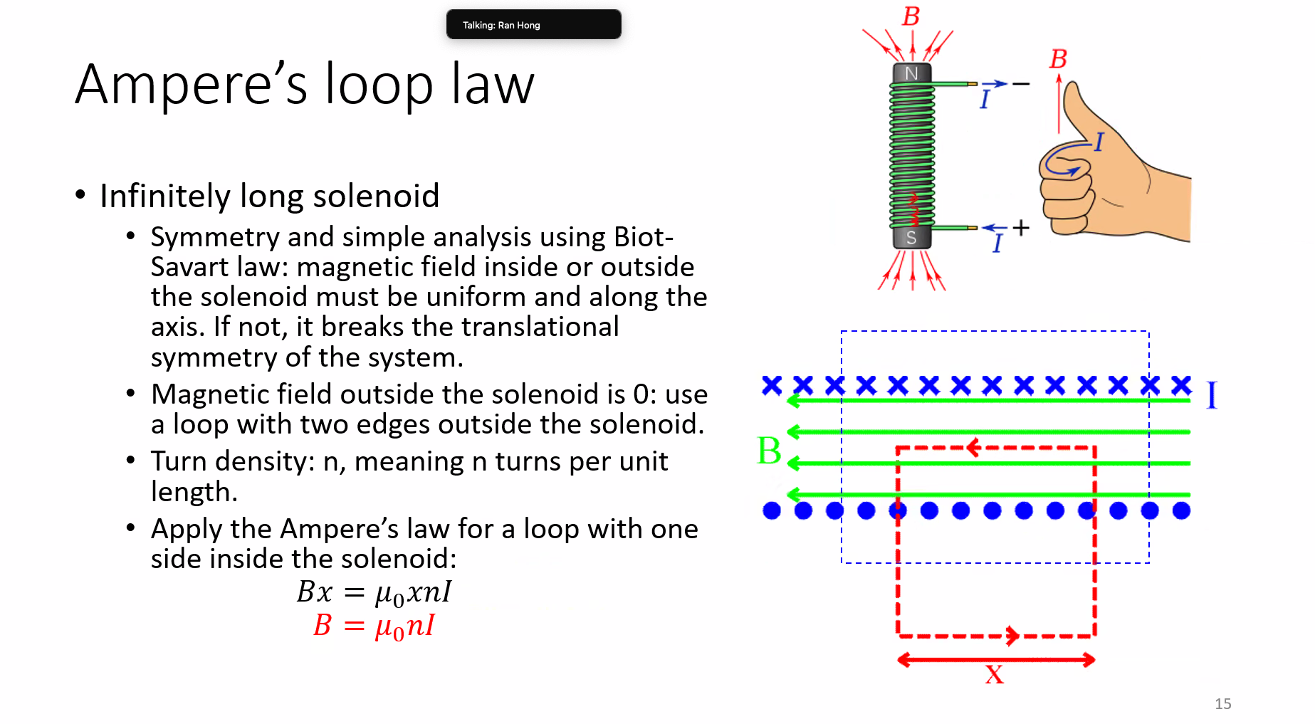
Proof (Field of an ideal solenoid). Model the winding as an infinitely long cylindrical current sheet. Symmetry gives an axial field. Rectangular Amperian loops with both long sides outside show that the external axial field is constant; requiring the solenoid’s field to vanish far away makes that constant zero. Loops entirely inside similarly give a uniform interior field.

Now choose a rectangular loop with one long side of length $\ell$ inside and the other outside. The short sides are perpendicular to the field. The surface cuts through $n\ell$ turns, so

$$B\ell=\mu_0(n\ell)I.$$

Therefore,

$$B_{\text{inside}}=\mu_0 nI,\qquad B_{\text{outside}}=0.$$

The direction follows your right thumb when your fingers curl along the winding current. A finite solenoid has a nonzero external field and end effects; the ideal result is a good approximation deep inside a long solenoid.

---

Magnetic force and charged-particle motion

The magnetic part of the Lorentz force is

$$\vec F_B=q\vec v\times\vec B, \qquad F_B=\lvert q\rvert vB\sin\theta.$$

Point your right index finger along $\vec v$ and your middle finger along $\vec B$. Your thumb gives the force on a positive charge. Reverse it for a negative charge.

The force is perpendicular to both $\vec v$ and $\vec B$, so

$$P_B=\vec F_B\cdot\vec v=0.$$

A magnetic field alone changes a particle’s direction, not its speed or kinetic energy. The full Lorentz force is $q(\vec E+\vec v\times\vec B)$; an electric field can do work, so the no-work statement applies only to the magnetic part.

Circular motion

If $\vec v\perp\vec B$ in a uniform field, the magnetic force supplies the centripetal force:

$$\lvert q\rvert vB=\frac{mv^2}{r},\qquad r=\frac{mv}{\lvert q\rvert B}=\frac{p}{\lvert q\rvert B}.$$

For nonrelativistic motion, the angular-frequency magnitude and period are

$$\omega_c=\frac{\lvert q\rvert B}{m}, \qquad T=\frac{2\pi m}{\lvert q\rvert B}.$$

The period does not depend on speed: faster particles trace proportionally larger circles. This speed independence is nonrelativistic; at relativistic speeds the period includes a factor of $\gamma$. The sign of $q$ determines the direction of rotation, not the sign of the radius or period.

Helical motion

Resolve the initial velocity into components parallel and perpendicular to the uniform field:

$$\vec v=\vec v_{\parallel}+\vec v_{\perp}.$$

The parallel component is unchanged because its cross product with $\vec B$ vanishes. The perpendicular component undergoes uniform circular motion. Combining them gives a helix with

$$r=\frac{mv_{\perp}}{\lvert q\rvert B}, \qquad T=\frac{2\pi m}{\lvert q\rvert B}, \qquad \text{pitch}=\lvert v_{\parallel}\rvert T.$$

If $v_{\parallel}=0$, the helix becomes a circle. If $v_{\perp}=0$, the path is straight along the field.

---

Force on a current-carrying wire

The force on a wire comes from the forces on its moving charge carriers. For a straight segment of length $L$ and cross-sectional area $A$, the number of carriers is $n_cAL$. Using their drift velocity and $\vec J=n_cq\vec v_d$ gives

$$\vec F=(n_cAL)q\vec v_d\times\vec B =I\vec L\times\vec B.$$

Here $\vec L$ points along conventional current, so the same formula works for positive or negative charge carriers. In magnitude,

$$F=ILB\sin\theta.$$

For a curved wire or a nonuniform field, add the forces on individual elements:

$$d\vec F=I\,d\vec\ell\times\vec B, \qquad \vec F=I\int_Cd\vec\ell\times\vec B.$$

Use the applied field at the wire, not the wire’s own singular idealized field. The force direction follows the same cross-product rule as for a positive charge: index finger along current, middle finger along field, thumb along force. Do not interchange current and field.

Torque on a loop

A closed loop in a uniform field has zero net force because

$$\vec F=I\left(\oint_Cd\vec\ell\right)\times\vec B=0.$$

The forces can still produce a torque.

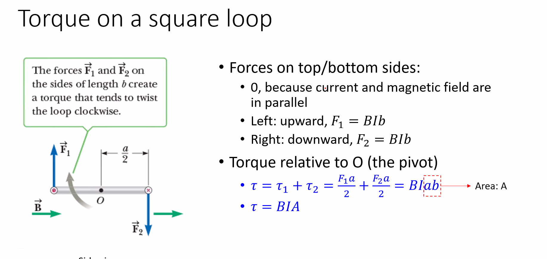
Proof (Torque on a rectangular loop). Let a rectangular loop have sides $a$ and $b$, so its area is $A=ab$. First put the field in the plane of the loop, parallel to the sides of length $a$. Those sides feel no force. The two sides of length $b$ feel opposite forces of magnitude $IBb$.

Each force has lever arm $a/2$ about the central pivot, giving

$$\tau=(IBb)\frac a2+(IBb)\frac a2=IBab=IAB.$$

When the loop’s normal makes angle $\theta$ with the field, the effective lever arm is reduced by $\sin\theta$:

$$\tau=IAB\sin\theta.$$

The angle is measured from the normal, not from the plane of the loop. The torque is largest when the field lies in the loop’s plane and zero when the normal is aligned with the field.

DC motor

The opposite forces on a current loop can turn a rotor. With a fixed current direction, the magnetic torque tries to align the loop’s magnetic moment with the field; it does not keep driving the rotation in the same sense through a full turn.

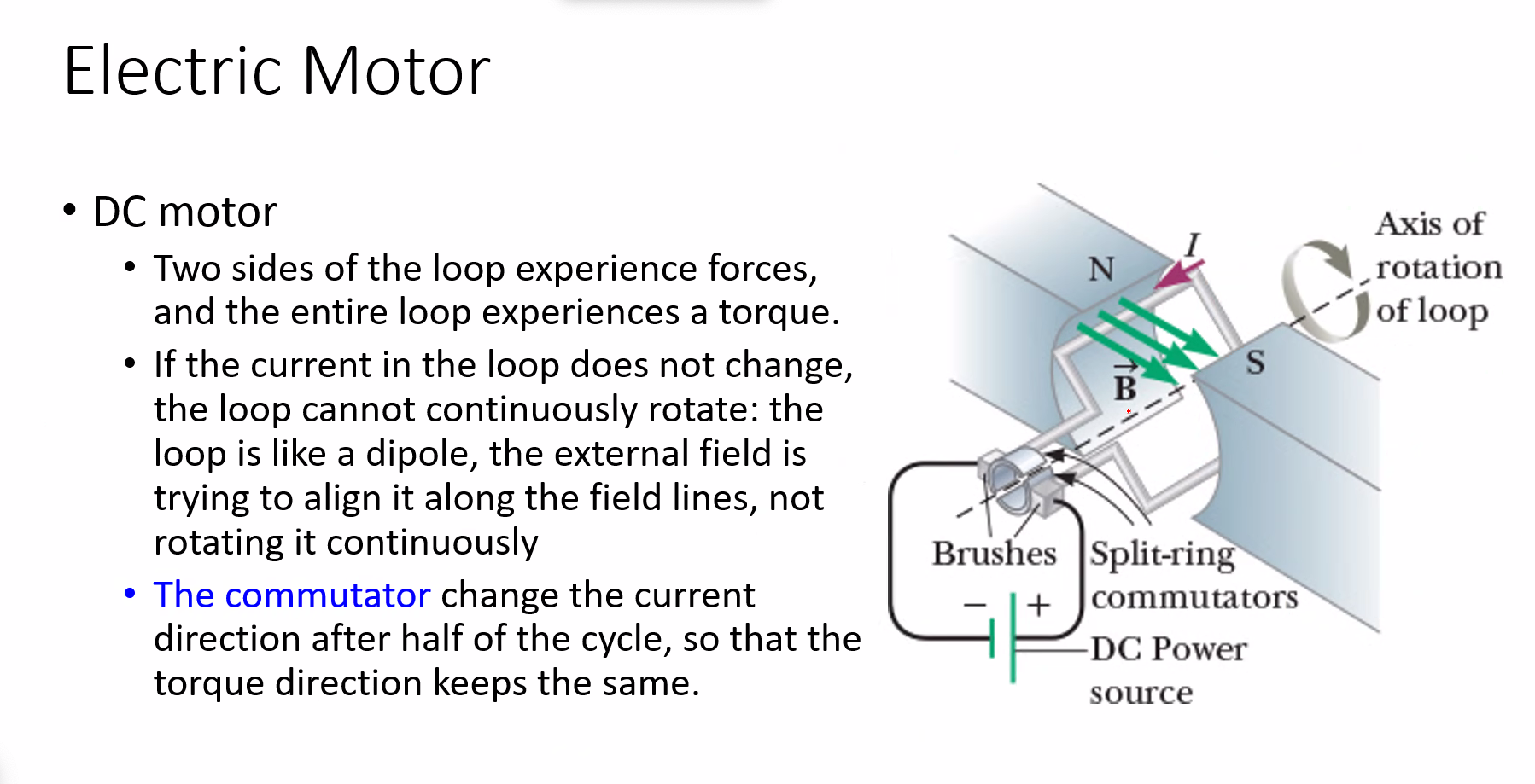
A split-ring commutator reverses the current every half-turn. This reverses the loop’s magnetic moment at the appropriate time, keeping the driving torque in the same rotational direction. Inertia carries the rotor through the orientations where the torque is momentarily zero.

---

Magnetic dipoles

A small current loop behaves as a magnetic dipole. For a planar loop, define

$$\vec m=IA\hat n.$$

Curl your right-hand fingers along the current; your thumb gives $\hat n$. This works for any planar loop shape, not just a rectangle. For $N$ identical aligned turns,

$$\vec m=NIA\hat n.$$

The unit is $\text{A}\cdot\text{m}^2$. Magnetic moment is often written $\vec\mu$, but we use $\vec m$ here to distinguish it from permeability $\mu$. Plain $m$ in the particle-motion section denotes mass.

Torque, energy, and force

In a uniform external field,

$$\vec\tau=\vec m\times\vec B, \qquad U=-\vec m\cdot\vec B=-mB\cos\theta.$$

The net force is zero, but the torque tends to align the moment with the field. Parallel alignment minimizes the energy; antiparallel alignment has zero torque but is unstable.

In a nonuniform field, a small dipole with fixed moment can experience a net force:

$$\vec F=\nabla(\vec m\cdot\vec B).$$

For $\vec m=m\hat x$ and a field along $\hat x$ on the dipole’s path,

$$F_x=m\frac{dB_x}{dx}.$$

An aligned fixed dipole is pulled toward stronger field. These energy and force expressions use an externally imposed field and a fixed moment; do not apply the fixed-moment derivative blindly to an induced moment that itself changes with position.

Field of a dipole

For the circular loop of radius $a$, $m=I\pi a^2$. Far along its positive axis, where $z\gg a$,

$$\vec B(z)\approx\frac{\mu_0 I a^2}{2z^3}\hat z =\frac{\mu_0 m}{2\pi z^3}\hat z.$$

At any point far from a localized dipole,

$$\vec B(\vec r)\approx\frac{\mu_0}{4\pi r^3} \left[3(\vec m\cdot\hat r)\hat r-\vec m\right].$$

If the moment points along positive $z$ and $\theta$ is the polar angle from that axis, this is

$$\vec B\approx\frac{\mu_0 m}{4\pi r^3} \left(2\cos\theta\,\hat r+\sin\theta\,\hat\theta\right).$$

On the equatorial plane the field points opposite $\vec m$, with half the axial magnitude at the same distance. The dipole approximation requires distance much larger than the source’s size.

For a localized steady current distribution, the general magnetic moment is

$$\vec m=\frac12\int_V\vec r\times\vec J(\vec r)\,dV.$$

---

Magnetism in materials

Atoms and molecules can have magnetic moments from electron orbital motion and intrinsic electron spin. Contributions often cancel, especially in filled shells. Spin is intrinsic angular momentum, not a little charged sphere literally rotating about an axis.

A magnet can be modeled as many microscopic dipoles. To find its total force or torque in an external field, add the contributions from those dipoles. Their average magnetic moment per unit volume is the magnetization:

$$\vec M=\frac{\sum_i\vec m_i}{\Delta V}.$$

The averaging volume is small on the scale of the object but contains many atoms. Magnetization has units $\text{A/m}$.

Paramagnetism

In a paramagnetic material, an applied field weakly favors alignment of microscopic moments along the field. Thermal motion prevents full alignment, so the average magnetization is usually small. Removing the field removes the preferred direction, and the bulk magnetization normally disappears.

Ferromagnetism and domains

In materials such as iron, nickel, and cobalt, neighboring moments can strongly favor parallel alignment. Regions with aligned moments are called magnetic domains. An unmagnetized sample can contain strongly magnetized domains pointing in different directions, with little net magnetization.

An applied field favors domains oriented along it. Domain walls move and moments rotate, producing a much larger response than ordinary paramagnetism.

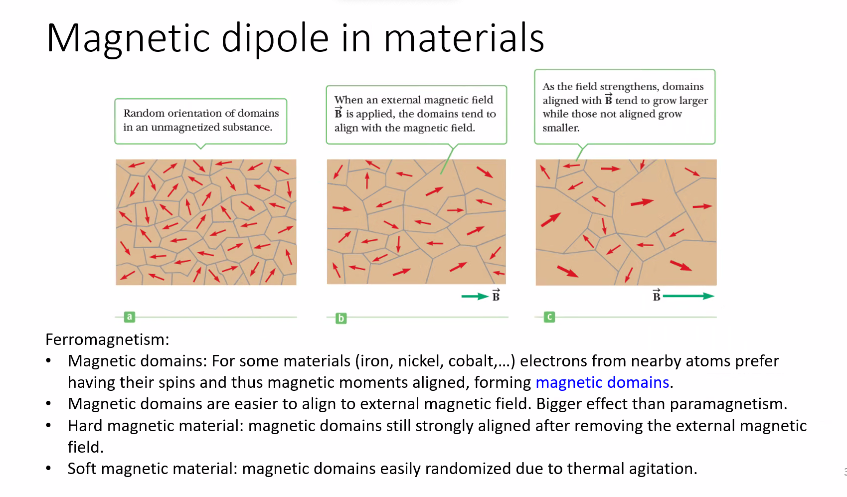
• Hard magnetic materials resist demagnetization and can retain substantial alignment after the field is removed. They are useful for permanent magnets.
• Soft magnetic materials are readily magnetized and demagnetized: their domain configuration changes under relatively small applied fields. This is not simply thermal randomization of all the moments.

Diamagnetism

An applied field also changes the orbital motion of electrons, inducing a magnetic response opposite to the applied field. This diamagnetic contribution occurs in all materials, but it is often hidden by stronger paramagnetic or ferromagnetic effects.

In materials such as copper and water, the diamagnetic response dominates. It is usually weak, although strong nonuniform fields can make its mechanical effects noticeable. Do not interpret the response as every electron simply beginning the same classical circular orbit; the orbital picture is a model for the induced opposing moment.

Superconductors and the Meissner effect

A superconductor supports persistent current without electrical resistance. In the Meissner state, screening currents near its surface expel magnetic flux from the bulk, so $\vec B\approx0$ well inside. The field penetrates a thin surface layer rather than stopping at a mathematically sharp boundary.

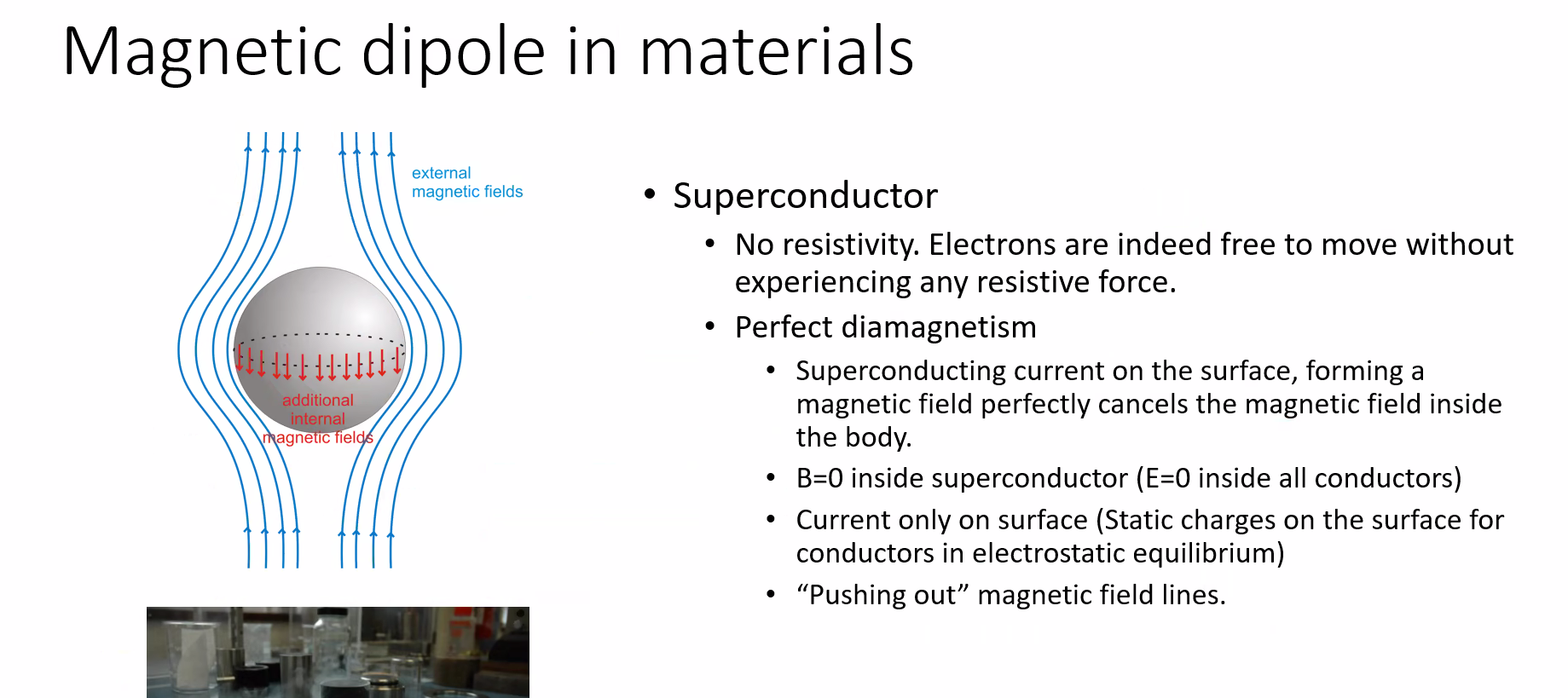
Type I superconductors lose superconductivity above a critical field. Type II superconductors also have a Meissner state below a lower critical field; between their lower and upper critical fields they enter a mixed state in which flux penetrates in vortices. Thus, “type II always freezes the field inside” is not a general rule. Zero resistance alone does not imply flux expulsion; the Meissner effect is an additional property. See the superconductivity discussion in OpenStax for this distinction.

---

Bound currents and the H-field

The microscopic current-loop model of magnetization can be replaced by equivalent bound currents. These describe the magnetic effect of the material’s dipoles, rather than a transport current supplied through a wire. The latter is a free current.

For magnetization $\vec M$, the bound surface and volume current densities are

$$\vec K_b=\vec M\times\hat n, \qquad \vec J_b=\nabla\times\vec M,$$

where $\hat n$ points outward from the material. If $\vec M$ is uniform inside the material, $\vec J_b=0$ there: neighboring microscopic loops cancel internally, leaving an equivalent surface current.

Example. A cylinder has uniform magnetization $\vec M=M\hat z$. Find its equivalent bound currents.

The volume current is zero because $\nabla\times\vec M=0$. On the curved surface, $\hat n=\hat r$, so

$$\vec K_b=M\hat z\times\hat r=M\hat\phi.$$

On the end faces, $\hat n=\pm\hat z$ and $\vec K_b=0$. The cylinder is therefore magnetically equivalent to an azimuthal surface current, like a solenoid winding.

Separating free and bound current

Ampère’s law counts both types of current:

$$\oint_C\vec B\cdot d\vec\ell =\mu_0(I_{f,\text{enc}}+I_{b,\text{enc}}).$$

The corresponding magnetization circulation gives the enclosed bound current, with surface contributions included at material boundaries:

$$I_{b,\text{enc}}=\oint_C\vec M\cdot d\vec\ell.$$

Moving this contribution to the left motivates the magnetic field strength $\vec H$:

$$\vec H=\frac{\vec B}{\mu_0}-\vec M, \qquad \oint_C\vec H\cdot d\vec\ell=I_{f,\text{enc}}.$$

Both $\vec H$ and $\vec M$ have units $\text{A/m}$. The field acting in the magnetic force law is still $\vec B$, not $\vec H$. In vacuum, $\vec M=0$ and $\vec B=\mu_0\vec H$.

Susceptibility and permeability

For a linear, isotropic magnetic material,

$$\vec M=\chi_m\vec H.$$

The dimensionless constant $\chi_m$ is the magnetic susceptibility. Substituting into the definition of $\vec H$ gives

$$\vec B=\mu_0(\vec H+\vec M) =\mu_0(1+\chi_m)\vec H=\mu\vec H,$$

where

$$\mu=\mu_0(1+\chi_m),\qquad \mu_r=\frac{\mu}{\mu_0}=1+\chi_m.$$

Paramagnets have $\chi_m>0$; diamagnets have $\chi_m<0$. For many ordinary weakly magnetic materials, $\lvert\chi_m\rvert\ll1$, so $\mu$ is close to $\mu_0$. The magnitude depends on material and temperature; a single small numerical range does not describe every paramagnet.

Ferromagnets can have a very large response, but a single constant $\chi_m$ or $\mu$ generally does not describe them. Their response is nonlinear and depends on the magnetization history.

Hysteresis

Increasing and then decreasing the applied field does not take a ferromagnet through the same sequence of domain configurations. A plot of $M$ against $H$, or $B$ against $H$, traces a hysteresis loop.

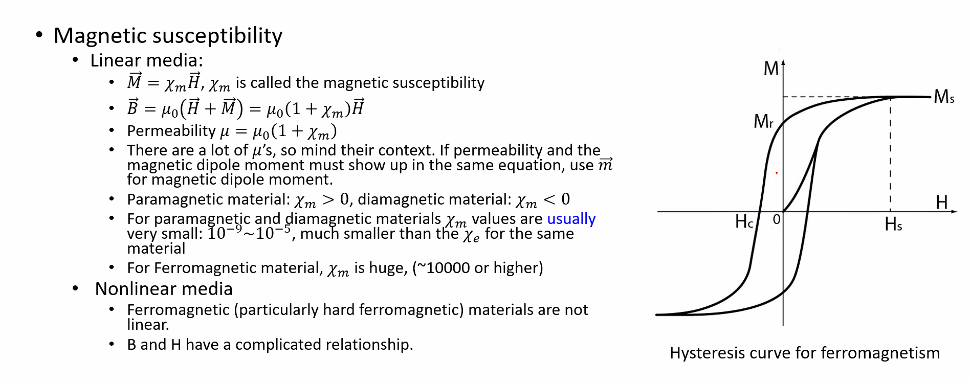
At large fields, the magnetization approaches saturation. After the field returns to zero, some magnetization can remain: remanence. A reverse field is needed to reduce the magnetization to zero; its magnitude is the coercive field for the $M$–$H$ loop. Hard magnets have high coercivity, while soft magnets have low coercivity. Distinguish an $M$–$H$ graph from a $B$–$H$ graph when reading its intercepts.

---

Equation summary

Key equations

Idea	Equation	Conditions / notation
Biot–Savart law	$d\vec B=\dfrac{\mu_0 I}{4\pi}\dfrac{d\vec\ell'\times\hat R}{R^2}$	Steady current in vacuum; $\vec R$ points from source to observation point
Infinite straight wire	$B=\dfrac{\mu_0 I}{2\pi r}$	$r$ is perpendicular distance from the wire
Circular loop on axis	$B_z=\dfrac{\mu_0 Ia^2}{2(a^2+z^2)^{3/2}}$	Radius $a$; sign follows current direction
Magnetic flux	$\Phi_B=\int_S\vec B\cdot d\vec A$	Uniform field and flat surface: $BA\cos\theta$
Gauss’s law / vector potential	$\oint_S\vec B\cdot d\vec A=0,\quad \nabla\cdot\vec B=0,\quad \vec B=\nabla\times\vec A$	Flux integral is over a closed surface
Ampère’s law	$\oint_C\vec B\cdot d\vec\ell=\mu_0 I_{\text{enc}}$	Magnetostatics; total signed enclosed current
Infinite current sheet	$B=\mu_0 K/2$	Equal magnitudes, opposite directions on the two sides
Uniform cylindrical wire	$B_{\text{in}}=\dfrac{\mu_0 Ir}{2\pi R^2},\quad B_{\text{out}}=\dfrac{\mu_0 I}{2\pi r}$	Inside $r\le R$; outside $r\ge R$
Ideal infinite solenoid	$B_{\text{in}}=\mu_0 nI,\quad B_{\text{out}}=0$	Vacuum core; $n$ turns per unit length
Magnetic force	$\vec F_B=q\vec v\times\vec B,\quad \vec F_B\cdot\vec v=0$	Reverse the positive-charge force for $q<0$
Circular / helical motion	$r=\dfrac{mv_\perp}{\lvert q\rvert B},\quad \omega_c=\dfrac{\lvert q\rvert B}{m},\quad T=\dfrac{2\pi m}{\lvert q\rvert B}$	Uniform field, nonrelativistic mass $m$; pitch $=\lvert v_\parallel\rvert T$
Wire force	$\vec F=I\int_Cd\vec\ell\times\vec B$	Straight wire in uniform field: $I\vec L\times\vec B$
Magnetic moment	$\vec m=NIA\hat n,\quad \vec m=\dfrac12\int_V\vec r\times\vec J\,dV$	Planar coil; general localized steady current, respectively
Dipole torque / energy	$\vec\tau=\vec m\times\vec B,\quad U=-\vec m\cdot\vec B$	Applied field; fixed magnetic moment
Dipole force	$\vec F=\nabla(\vec m\cdot\vec B),\quad F_x=m\,dB_x/dx$	Small fixed dipole; second form for alignment along $x$
Far dipole field	$\vec B\approx\dfrac{\mu_0}{4\pi r^3}[3(\vec m\cdot\hat r)\hat r-\vec m]$	Distance much larger than source size
Magnetization / bound current	$\vec M=\dfrac{\sum_i\vec m_i}{\Delta V},\quad\vec K_b=\vec M\times\hat n,\quad\vec J_b=\nabla\times\vec M$	$\hat n$ is outward normal
H-field	$\vec H=\vec B/\mu_0-\vec M,\quad\oint_C\vec H\cdot d\vec\ell=I_{f,\text{enc}}$	Magnetostatics; only free current on the right
Linear magnetic medium	$\vec M=\chi_m\vec H,\quad\vec B=\mu\vec H,\quad\mu=\mu_0(1+\chi_m)$	Linear, isotropic response; not a general ferromagnet law